Multivariate normal distribution
Probability density function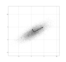 Multivariate (bivariate) Gaussian distribution centered at (1,3) with a standard deviation of 3 in roughly the (0.878, 0.478) direction and of 1 in the orthogonal direction. |
|
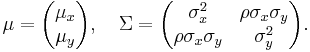
| parameters: | μ ∈ Rk — location Σ ∈ Rk×k — covariance (nonnegative-definite matrix) |
|---|---|
| support: | x ∈ span(Σ) ⊆ Rk |
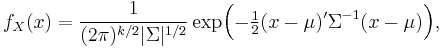
| pdf: | 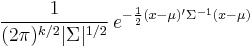 (pdf exists only for positive-definite Σ) |
| cdf: | (no analytic expression) |
| mean: | μ |
| mode: | μ |
| variance: | Σ |
| entropy: | 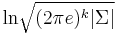 |
| mgf: | 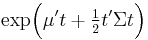 |
| cf: |  |
In probability theory and statistics, the multivariate normal distribution or multivariate Gaussian distribution, is a generalization of the one-dimensional (univariate) normal distribution to higher dimensions. A random vector is said to be multivariate normally distributed if every linear combination of its components has a univariate normal distribution.
Notation and parametrization
The multivariate normal distribution of a k-dimensional random vector ![X = [X_1, X_2, \ldots, X_k]](/2010-wikipedia_en_wp1-0.8_orig_2010-12/I/4fc06040a228f8ba3919c1d397538f71.png) can be written in the following notation:
can be written in the following notation:
or to make it explicitly known that X is k-dimensional,
with k-dimensional mean vector
![\mu = [ \operatorname{E}[X_1], \operatorname{E}[X_2], \ldots, \operatorname{E}[X_k]]](/2010-wikipedia_en_wp1-0.8_orig_2010-12/I/4f60085a79edcd2c98f8ef0e1ee56c65.png)
and k x k covariance matrix
![\Sigma = [\operatorname{Cov}[X_i, X_j]]_{i=1,2,\ldots,k; j=1,2,\ldots,k}](/2010-wikipedia_en_wp1-0.8_orig_2010-12/I/3ba5d0c02c197292637d26dfe6f9a3f2.png)
Definition
A random vector X = (X1, …, Xk)′ is said to have the multivariate normal distribution if it satisfies the following equivalent conditions [1]:
- Every linear combination of its components Y = a1X1 + … + akXk is normally distributed. That is, for any constant vector a ∈ Rk, the random variable Y = a′X has a univariate normal distribution.
- There exists a random ℓ-vector Z, whose components are independent normal random variables, a k-vector μ, and a k×ℓ matrix A, such that X = AZ + μ. Here ℓ is the rank of the covariance matrix Σ = AA′.
- There is a k-vector μ and a symmetric, nonnegative-definite k×k matrix Σ, such that the characteristic function of X is
- (Only in case when the support of X is the entire space Rk). There exists a k-vector μ and a symmetric positive-definite k×k matrix Σ, such that the probability density function of X can be expressed as
The covariance matrix is allowed to be singular (in which case the corresponding distribution has no density). This case arises frequently in statistics; for example, in the distribution of the vector of residuals in the ordinary least squares regression. Note also that the Xi are in general not independent; they can be seen as the result of applying the matrix A to a collection of independent Gaussian variables Z.
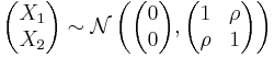
Bivariate case
In the 2-dimensional nonsingular case (k = rank(Σ) = 2), the probability density function of a vector [X Y]′ is
![f(x,y) =
\frac{1}{2 \pi \sigma_x \sigma_y \sqrt{1-\rho^2}}
\exp\left(
-\frac{1}{2(1-\rho^2)}\left[
\frac{(x-\mu_x)^2}{\sigma_x^2} +
\frac{(y-\mu_y)^2}{\sigma_y^2} -
\frac{2\rho(x-\mu_x)(y-\mu_y)}{\sigma_x \sigma_y}
\right]
\right),](/2010-wikipedia_en_wp1-0.8_orig_2010-12/I/b10ecc56f758b2f94a953e7e1bd2f1c2.png)
where ρ is the correlation between X and Y. In this case,
In the bivariate case, we also have a theorem that makes the first equivalent condition for multivariate normality less restrictive: it is sufficient to verify that countably many distinct linear combinations of X and Y are normal in order to conclude that the vector [X Y]′ is bivariate normal.[2]
Properties
Cumulative distribution function
The cumulative distribution function (cdf) F(x) of a random vector X is defined as the probability that all components of X are less than or equal to the corresponding values in the vector x. Though there is no closed form for F(x), there are a number of algorithms that estimate it numerically. For example, see MVNDST under [2] (includes FORTRAN code) or [3] (includes MATLAB code).
Normally distributed and independent
If X and Y are normally distributed and independent, this implies they are "jointly normally distributed", i.e., the pair (X, Y) must have bivariate normal distribution. However, a pair of jointly normally distributed variables need not be independent.
Two normally distributed random variables need not be jointly bivariate normal
The fact that two random variables X and Y both have a normal distribution does not imply that the pair (X, Y) has a joint normal distribution. A simple example is one in which X has a normal distribution with expected value 0 and variance 1, and Y = X if |X| > c and Y = −X if |X| < c, where c is about 1.54. There are similar counterexamples for more than two random variables.
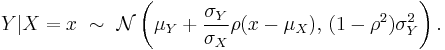
Conditional distributions
If  and
and  are partitioned as follows
 with sizes
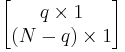
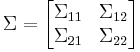 with sizes
then the distribution of  conditional on
  is multivariate normal
 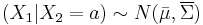 where
where
and covariance matrix
This matrix is the Schur complement of  in
in  . This means that to calculate the conditional covariance matrix, one inverts the overall covariance matrix, drops the rows and columns corresponding to the variables being conditioned upon, and then inverts back to get the conditional covariance matrix.
Note that knowing that alters the variance, though the new variance does not depend on the specific value of  ; perhaps more surprisingly, the mean is shifted by
 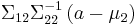 ; compare this with the situation of not knowing the value of , in which case would have distribution
  .
.
The matrix  is known as the matrix of regression coefficients.
In the bivariate case the conditional distribution of Y given X is
Bivariate conditional expectation
In the case
then
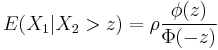
where this latter ratio is often called the inverse Mills ratio.
Marginal distributions
To obtain the marginal distribution over a subset of multivariate normal random variables, one only needs to drop the irrelevant variables (the variables that one wants to marginalize out) from the mean vector and the covariance matrix. The proof for this follows from the definitions of multivariate normal distributions and some advanced linear algebra [3].
Example
Let ![X =[X_1, X_2, X_3]](/2010-wikipedia_en_wp1-0.8_orig_2010-12/I/e6f8db6a40172eac50975bb5cb08fcd6.png) be multivariate normal random variables with mean vector
be multivariate normal random variables with mean vector ![\mu = [\mu_1 \mu_2 \mu_3]](/2010-wikipedia_en_wp1-0.8_orig_2010-12/I/2ad42833f81238471ceba99b9478d4af.png) and covariance matrix (Standard parametrization for multivariate normal distribution). Then the joint distribution of
and covariance matrix (Standard parametrization for multivariate normal distribution). Then the joint distribution of ![X' = [X_1 X_3]](/2010-wikipedia_en_wp1-0.8_orig_2010-12/I/a9a7565eb2ae415b9d02b27f415914b1.png) is multivariate normal with mean vector
is multivariate normal with mean vector ![\mu' = [\mu_1 \mu_3]](/2010-wikipedia_en_wp1-0.8_orig_2010-12/I/346f3f3dd16318768150c2f38d0f7e46.png) and covariance matrix
and covariance matrix 
Affine transformation
If  is an affine transformation of
  where
where  is an
is an  vector of constants and
  is a constant
  matrix, then
  has a multivariate normal distribution with expected value
  and variance
  i.e.,
i.e.,  . In particular, any subset of the
  has a marginal distribution that is also multivariate normal. To see this, consider the following example: to extract the subset
  , use
, use
which extracts the desired elements directly.
Another corollary is that the distribution of  , where
  is a constant vector of the same length as
  and the dot indicates a vector product, is univariate Gaussian with
  . This result follows by using
and considering only the first component of the product (the first row of  is the vector ). Observe how the positive-definiteness of implies that the variance of the dot product must be positive.
An affine transformation of such as  is not the same as the sum of two independent realisations of .
Geometric interpretation
The equidensity contours of a non-singular multivariate normal distribution are ellipsoids (i.e. linear transformations of hyperspheres) centered at the mean[4]. The directions of the principal axes of the ellipsoids are given by the eigenvectors of the covariance matrix . The squared relative lengths of the principal axes are given by the corresponding eigenvalues.
If 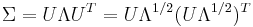 is an eigendecomposition where the columns of U are unit eigenvectors and
  is a diagonal matrix of the eigenvalues, then we have

Moreover, U can be chosen to be a rotation matrix, as inverting an axis does not have any effect on  , but inverting a column changes the sign of U's determinant. The distribution
  is in effect
  scaled by
  , rotated by U and translated by .
Conversely, any choice of , full rank matrix U, and positive diagonal entries  yields a non-singular multivariate normal distribution. If any is zero and U is square, the resulting covariance matrix
  is singular. Geometrically this means that every contour ellipsoid is infinitely thin and has zero volume in n-dimensional space, as at least one of the principal axes has length of zero.
Correlations and independence
In general, random variables may be uncorrelated but highly dependent. But if a random vector has a multivariate normal distribution then any two or more of its components that are uncorrelated are independent. This implies that any two or more of its components that are pairwise independent are independent.
But it is not true that two random variables that are (separately, marginally) normally distributed and uncorrelated are independent. Two random variables that are normally distributed may fail to be jointly normally distributed, i.e., the vector whose components they are may fail to have a multivariate normal distribution. For an example of two normally distributed random variables that are uncorrelated but not independent, see normally distributed and uncorrelated does not imply independent.
Higher moments
The kth-order moments of X are defined by
![\mu _{1,\dots,N}(X)\ \stackrel{\mathrm{def}}{=}\ \mu _{r_{1},\dots,r_{N}}(X)\ \stackrel{\mathrm{def}}{=}\ E\left[
\prod\limits_{j=1}^{N}X_j^{r_{j}}\right]](/2010-wikipedia_en_wp1-0.8_orig_2010-12/I/8e895d7ed390749881b8992984ae3fa8.png)
where 
The central k-order central moments are given as follows
(a) If k is odd,  .
.
(b) If k is even with  , then

where the sum is taken over all allocations of the set  into
into  (unordered) pairs. That is, if you have a kth (
 ) central moment, you will be summing the products of
  covariances (the - notation has been dropped in the interests of parsimony):
![\begin{align}
& {} E[X_1 X_2 X_3 X_4 X_5 X_6] \\
&{} = E[X_1 X_2 ]E[X_3 X_4 ]E[X_5 X_6 ] + E[X_1 X_2 ]E[X_3 X_5 ]E[X_4 X_6] + E[X_1 X_2 ]E[X_3 X_6 ]E[X_4 X_5] \\
&{} + E[X_1 X_3 ]E[X_2 X_4 ]E[X_5 X_6 ] + E[X_1 X_3 ]E[X_2 X_5 ]E[X_4 X_6 ] + E[X_1 X_3]E[X_2 X_6]E[X_4 X_5] \\
&+ E[X_1 X_4]E[X_2 X_3]E[X_5 X_6]+E[X_1 X_4]E[X_2 X_5]E[X_3 X_6]+E[X_1 X_4]E[X_2 X_6]E[X_3 X_5] \\
& + E[X_1 X_5]E[X_2 X_3]E[X_4 X_6]+E[X_1 X_5]E[X_2 X_4]E[X_3 X_6]+E[X_1 X_5]E[X_2 X_6]E[X_3 X_4] \\
& + E[X_1 X_6]E[X_2 X_3]E[X_4 X_5 ] + E[X_1 X_6]E[X_2 X_4 ]E[X_3 X_5] + E[X_1 X_6]E[X_2 X_5]E[X_3 X_4].
\end{align}](/2010-wikipedia_en_wp1-0.8_orig_2010-12/I/477220038abb3f6d2ee172e33bcde13f.png)
This yields  terms in the sum (15 in the above case), each being the product of (in this case 3) covariances. For fourth order moments (four variables) there are three terms. For sixth-order moments there are 3 × 5 = 15 terms, and for eighth-order moments there are 3 × 5 × 7 = 105 terms.
The covariances are then determined by replacing the terms of the list ![\left[ 1,\dots,2\lambda \right]](/2010-wikipedia_en_wp1-0.8_orig_2010-12/I/218c7d67059fcf04a548d845d9f6e1d7.png) by the corresponding terms of the list consisting of
by the corresponding terms of the list consisting of  ones, then
  twos, etc... To illustrate this, examine the following 4th-order central moment case:
![E\left[ X_i^4\right] = 3\sigma _{ii}^2](/2010-wikipedia_en_wp1-0.8_orig_2010-12/I/7ee572fbf3fbe2077e2f886d7710d1d4.png)
![E\left[ X_i^3 X_j\right] = 3\sigma _{ii} \sigma _{ij}](/2010-wikipedia_en_wp1-0.8_orig_2010-12/I/bd7a84adc118f6fef0d3e44fd515f707.png)
![E\left[ X_i^2 X_j^2\right] = \sigma _{ii}\sigma_{jj}+2\left( \sigma _{ij}\right) ^2](/2010-wikipedia_en_wp1-0.8_orig_2010-12/I/4b34e16082722ca5e14bc525aa275597.png)
![E\left[ X_i^2X_jX_k\right] = \sigma _{ii}\sigma _{jk}+2\sigma _{ij}\sigma _{ik}](/2010-wikipedia_en_wp1-0.8_orig_2010-12/I/ea55493c283fd864bcbe46c5da9c4ee5.png)
![E\left[ X_i X_j X_k X_n\right] = \sigma _{ij}\sigma _{kn}+\sigma _{ik}\sigma _{jn}+\sigma _{in}\sigma _{jk}.](/2010-wikipedia_en_wp1-0.8_orig_2010-12/I/67659b5bf0652636330890c6b45712d7.png)
where  is the covariance of
  and
and  . The idea with the above method is you first find the general case for a
  th moment where you have different variables -
 ![E\left[ X_i X_j X_k X_n\right]](/2010-wikipedia_en_wp1-0.8_orig_2010-12/I/cf7446bc0444c0d68bd8dd68dd68a195.png) and then you can simplify this accordingly. Say, you have
and then you can simplify this accordingly. Say, you have ![E\left[ X_i^2 X_k X_n\right]](/2010-wikipedia_en_wp1-0.8_orig_2010-12/I/bdf61709456f398f3ff0535c90a2da35.png) then you simply let
then you simply let  and realise that
  .
.
Kullback–Leibler divergence
The Kullback–Leibler divergence from  to
to  , for non-singular matrices
  and
and  , is:
, is:

The logarithm must be taken to base e since the two terms following the logarithm are themselves base-e logarithms of expressions that are either factors of the density function or otherwise arise naturally. The equation therefore gives a result measured in nats. Dividing the entire expression above by loge 2 yields the divergence in bits.
Estimation of parameters
The derivation of the maximum-likelihood estimator of the covariance matrix of a multivariate normal distribution is perhaps surprisingly subtle and elegant. See estimation of covariance matrices.
In short, the probability density function (pdf) of an N-dimensional multivariate normal is

and the ML estimator of the covariance matrix from a sample of n observations is
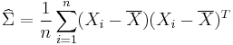
which is simply the sample covariance matrix. This is a biased estimator whose expectation is
![E[\widehat\Sigma] = {n-1 \over n}\Sigma.](/2010-wikipedia_en_wp1-0.8_orig_2010-12/I/6f5b2fd1317b7743d57df74a3e9350dc.png)
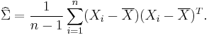
An unbiased sample covariance is
The Fisher information matrix for estimating the parameters of a multivariate normal distribution has a closed form expression. This can be used, for example, to compute the Cramer-Rao bound for parameter estimation in this setting. See Fisher information#Multivariate normal distribution for more details.
Entropy
The differential entropy of the multivariate normal distribution is [6]
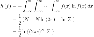
where  is the determinant of the covariance matrix .
Multivariate normality tests
Multivariate normality tests check a given set of data for similarity to the multivariate normal distribution. The null hypothesis is that the data set is similar to the normal distribution, therefore a sufficiently small p-value indicates non-normal data. Multivariate normality tests include the Cox-Small test [7] and Smith and Jain's adaptation [8] of the Friedman-Rafsky test.[9]
Drawing values from the distribution
A widely used method for drawing a random vector from the  -dimensional multivariate normal distribution with mean vector and covariance matrix (required to be symmetric and positive-definite) works as follows:
- Find any matrix A such that
 . Often this is a Cholesky decomposition, though a square root of would also suffice.
 - Let
 be a vector whose components are independent standard normal variates (which can be generated, for example, by using the Box-Muller transform).
 - Let
 be
be  . This has the desired distribution due to the affine transformation property.
See also
- Chi distribution, the pdf of the 2-norm (or Euclidean norm) of a multivariate normally-distributed vector.
References
- ↑ Gut, Allan: An Intermediate Course in Probability, 2009, chapter 5
- ↑ Hamedani & Tata (1975)
- ↑ The formal proof for marginal distribution is shown here http://fourier.eng.hmc.edu/e161/lectures/gaussianprocess/node7.html
- ↑ Nikolaus Hansen. "The CMA Evolution Strategy: A Tutorial" (PDF). http://www.bionik.tu-berlin.de/user/niko/cmatutorial.pdf.
- ↑ Penny & Roberts, PARG-00-12, (2000) [1]. pp. 18
- ↑ Gokhale, DV; NA Ahmed, BC Res, NJ Piscataway (May 1989). "Entropy Expressions and Their Estimators for Multivariate Distributions". Information Theory, IEEE Transactions on 35 (3): 688–692. doi:10.1109/18.30996.
- ↑ Cox, D. R.; N. J. H. Small (August 1978). "Testing multivariate normality". Biometrika 65 (2): 263–272. doi:10.1093/biomet/65.2.263.
- ↑ Smith, Stephen P.; Anil K. Jain (September 1988). "A test to determine the multivariate normality of a dataset". IEEE Transactions on Pattern Analysis and Machine Intelligence 10 (5): 757–761. doi:10.1109/34.6789.
- ↑ Friedman, J. H. and Rafsky, L. C. (1979) "Multivariate generalizations of the Wald-Wolfowitz and Smirnov two sample tests". Annals of Statistics, 7, 697–717.
Literature
Hamedani, G. G.; Tata, M. N. (1975). "On the determination of the bivariate normal distribution from distributions of linear combinations of the variables". The American Mathematical Monthly (The American Mathematical Monthly, Vol. 82, No. 9) 82 (9): 913–915. doi:10.2307/2318494. JSTOR 2318494. http://jstor.org/stable/2318494.
|
||||||||||||||||||||||||||||||||||||||||||||||||||||||||||||||||||